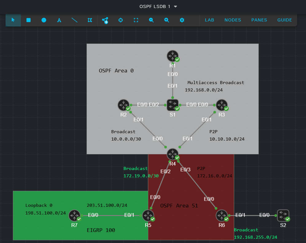
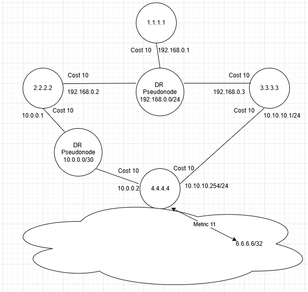
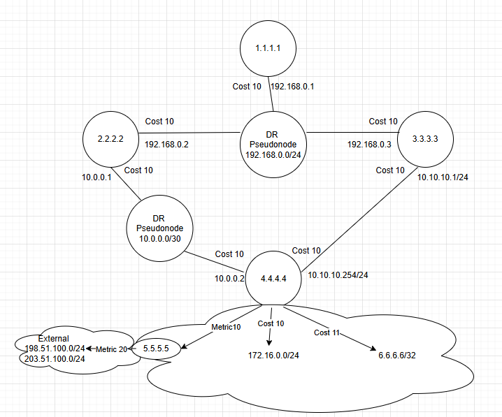
In this lab exercise, I am going to attempt to draw a diagram of the network based on the OSPF Link State Database (LSDB) using the virtualized network shown below. The diagram will be based on R1’s view of the network. R1’s OSPF Router ID (RID) is 1.1.1.1.
Let’s start by examining R1s LSDB at a high level using the command shown.

We can glean a lot of information about the network from this high level LSDB snapshot. We can immediately see that R1’s area, area 0, has 4 routers participating in OSPF. This is known because there are 4 Router LSAs displayed. This output also confirms that area 0 has two broadcast segments as confirmed by the two Type 2 (AKA Network) LSAs. We know that there is at least 1 non-backbone area because Type 3 (AKA Summary) LSAs exist. The presence of Type 5 LSAs confirms that routes are being redistributed into OSPF, and the Type 4 LSA confirms that redistribution is occurring outside of area 0.
Next, let’s check out R1’s self-originated type 1 LSA, also known as the Router LSA using the command shown.
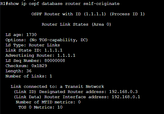
From this output, we confirm that R1’s OSPF Router ID (RID) is 1.1.1.1 and that it is connected to a transit, broadcast network with a cost of 10. We can also see that R1’s interface on this broadcast segment is 192.168.0.1 and that there is a Designated Router (DR) with an IP address of 192.168.0.3.
Let’s start out LSDB diagram by adding 1.1.1.1 and the information we know so far.

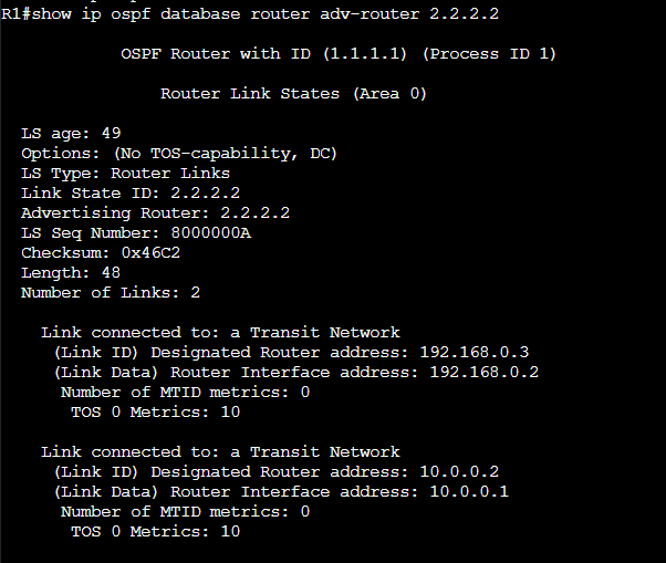
The high level LSDB output we saw earlier shows that there are 4 routers within the same area as R1. Let’s next view the Router LSAs originated by 2.2.2.2 using the command shown.

We can see here that 2.2.2.2 is also connected to a broadcast, transit segment using IP address 192.168.0.2 where 192.168.0.3 is the DR. We can see that 2.2.2.2 is also connected to a different transit, broadcast segment using IP address 10.0.0.1 where the DR has IP address 10.0.0.2. We don’t have enough information yet to add 2.2.2.2 to our diagram. Let’s press on for now and check out 3.3.3.3’s Router LSAs.

We have yet another similarity in 3.3.3.3’s router LSA. 3.3.3.3 is connected to a transit, broadcast segment using IP address 192.168.0.3 where 192.168.0.3 is the Designated Router. This gives us a clue that 3.3.3.3 is the DR on the segment where it is using IP 192.168.0.3. Those last two entries represent a point-to-point segment between 3.3.3.3 and 4.4.4.4 using IP network 10.10.10.0/24 where RID 3.3.3.3 is using IP 10.10.10.1 on the segment with a cost of 10.
Before we add 3.3.3.3 to our diagram, let’s examine the Type 2 (Network) LSA originated by 3.3.3.3. The network LSA is only originated by designated routers.
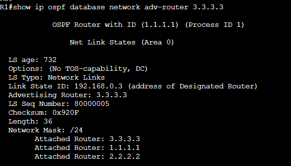
We can see in the type 2 LSA above that 1.1.1.1, 2.2.2.2, and 3.3.3.3 are connected to a common broadcast segment. The network LSA confirms again that 3.3.3.3 is connected to the shared segment with IP address 192.168.0.3, we can also see that the subnet mask of the link is 255.255.255.0. Combining this information with the Router LSA output we saw previously, we can add 2.2.2.2 and 3.3.3.3 to our diagram.
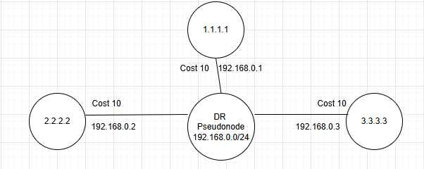
In my mind, the DR represents the multiaccess segment as a virtual node at the center of the segment with all other participating routers connected. This transforms what would be a full mesh of adjacencies into a hub and spoke. This is an optimization for SPF calculation. There are also update and hello flooding optimizations included with the DR that are outside the scope of this article.
Let’s now jump back to observing 3.3.3.3’s Router LSA. Below is a repost of the same screenshot we saw previously.
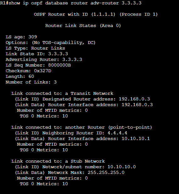
The 1st entry is already on our diagram so let’s focus on the 2nd two. Both represent a point-to-point network. We can see that the neighboring router is 4.4.4.4 and that 3.3.3.3 is using IP address 10.10.10.1 on this link. The next entry lets us know that the network ID is 10.10.10.0 with a 24-bit subnet mask. We can also see that 3.3.3.3 has a cost of 10 for this link. Let’s add 4.4.4.4 to our diagram based on what we know.

We don’t yet know what 4.4.4.4’s cost is on the link to 3.3.3.3, nor do we know its IP address. We’ll see that later when we view 4.4.4.4’s Router LSA.
Let’s now jump back to 2.2.2.2 and look closer at the Router LSA. Below is a repost of the previous screenshot. We know from this output that 2.2.2.2 is connected to another segment that appears to be broadcast, indicated by the presence of a DR. We know what 2.2.2.2 is not the DR because the Router Interface and Designated Router IP addresses do not match.
Let’s view our LSDB overview screenshot again.

4.4.4.4 is originating a Network LSA (type 2) with link ID 10.0.0.2. This is likely a broadcast segment connecting 2.2.2.2 and 4.4.4.4. Let’s drill in on 4.4.4.4’s Network LSA.

That’s it! This data lets us know that 2.2.2.2 and 4.4.4.4 do indeed share a broadcast segment and that no other routers exist on the link. We can see in this data that the IP address of the DR is 10.0.0.2 and that the subnet mask is 255.255.255.252. Let’s view 4.4.4.4’s Router LSA to get the full picture and add this segment to our diagram.

Let’s only pay attention to the 3rd entry for now. This confirms that 4.4.4.4 has IP address 10.0.0.2 (that we saw earlier is the DR IP on the segment connection to 2.2.2.2). We also now know that 4.4.4.4 has a cost of 10 on this segment.
We have enough data to represent the broadcast segment between 2.2.2.2 and 4.4.4.4.

Before we move on, let’s briefly revisit 4.4.4.4’s Router LSA.
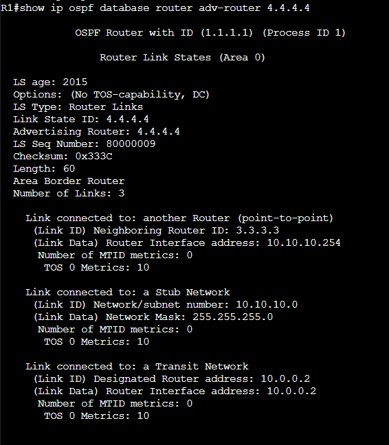
Those first two entries we skipped over earlier let us complete the diagram for the P2P link to 3.3.3.3. We can see 4.4.4.4’s interface IP and cost for the segment. 4.4.4.4’s IP address is 10.10.10.254 and the metric is 10.

Ok, now what? Let’s take a look at the high level LSDB again and see what we should investigate next.
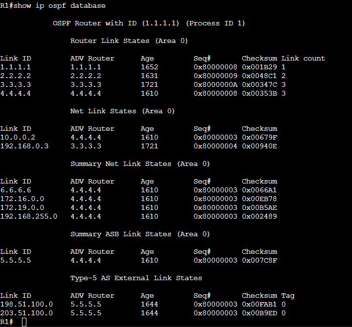
We have now viewed all the Router LSAs that R1 is privy to. Recall that Router LSAs are not flooded beyond area boundaries. We can conclude that only 1.1.1.1, 2.2.2.2, 3.3.3.3, and 4.4.4.4 participate in area 0.
We can now start with the Type 3, Summary LSAs. This name can be misleading. The Summary LSA does not necessarily advertise aggregated blocks of IP addresses. They are called Summary LSAs because they advertise summarized topology information. Area 0 does not have detailed topology information for other areas; the Area Border Router (ABR) summarizes information into other areas. Hopefully these next demonstrations will solidify this concept. Recall that we are attempting to diagram the network as seen from R1’s LSDB. We will not be able to see the specifics of Area 51 here. The output above shows us that only 4.4.4.4 is originating summary LSAs. It must be the only ABR.
Let’s drill into the Summary LSAs on R1 using the command shown. The output was too much to fit on 1 screen so the screenshot is broken up into two parts.


There is a lot of data here so let’s start by reviewing the first entry in detail.

Here we can see that the LS type is Summary, the Link State ID (network subnet) is 6.6.6.6 with a /32 mask. We see also that the Advertising Router is 4.4.4.4. The Metric displayed here is 11, this is the metric FROM the advertising router to the destination network. For R1 to calculate the total distance to 6.6.6.6/62, it will have to calculate the best distance to 4.4.4.4 and then add 11 to that metric. This is an example of topology summarization. From R1’s perspective, we don’t know the entire topology to reach 6.6.6.6/32. We only know that this network has a metric of 11 from the ABR. The ABR has an interface in area 0 so R1 can use type 1 and type 2 LSAs to find the path to the ABR. This routing paradigm is more distance vector like.
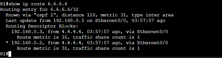
R1 has a total cost of 31 to reach 6.6.6.6. 20 to reach 4.4.4.4, and 11 from 4.4.4.4 to IP address 6.6.6.6/32.
I drew the non-backbone area as a cloud since R1 cannot see the topological detail.
I won’t drag you through all of the Summary LSAs but I will add one more, the next entry shown below.
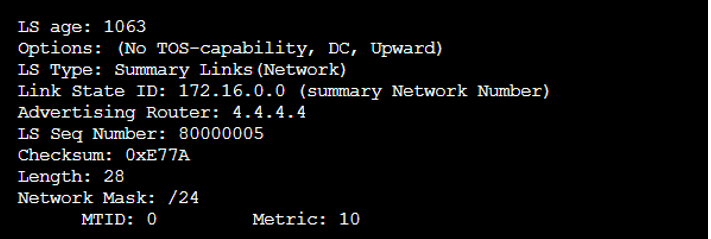
Again, this is the Summary advertisement from 4.4.4.4. All that R1 can see is that 4.4.4.4 can get us to 172.16.0.0/24 and that the cost FROM 4.4.4.4 is 10.

I was intentional about using unidirectional arrows here. The cost may not be the same in both directions. They typically are, but do not have to be.
We’ve now worked through the type 1, 2 and some of the type 3 LSAs in R1’s LSDB. Let’s pivot to viewing the LSAs that help R1 reach the external networks that are being redistributed into Area 51.

This output gives us some great information. The Link State ID in this output is the network ID of the external network that is redistributed into OSPF. We can also see the subnet mask, metric type, and metric. The Metric Type is either 1 or 2. Metric type 1 will represent the cumulative cost to reach the external destination. Metric type 2 is different. Metric type 2 does not increase as the LSA propagates further from its origination point. The metric will remain whatever it is set to at the Autonomous System Boundary Router (ASBR). The ASBR is the router that is redistributing information into OSPF.
A critical thing to understand about Type 5 LSAs is that the metric displayed is the metric as seen by the ASBR. This does not necessarily represent the full path metric for a metric type 1 external route.
The elephant in the room with these Type 5 LSAs is the Advertising Router ID. In this example, the Advertising Router is 5.5.5.5. We have not seen this RID yet. Recall that R1 does not have a router LSA for 5.5.5.5, so with what we have seen so far, R1 has no idea how to reach these external networks.
The additions to the diagram display what R1 knows about the external networks based on the information in the Type 5. Note that there is no known reachability to 5.5.5.5

The Type 4 LSA will help R1 and all other routers in area 0 reach these external networks. Let’s view it next.
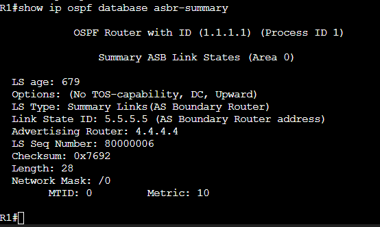
This is the glue that connects Area 0 to the Type 5 External Routes we just saw. The ABR, 4.4.4.4 generates this Type 4 and injects it into area 0. This type 4 lets Area 0 know that “you can reach 5.5.5.5 though me. My cost to get to 5.5.5.5 is 10.” 4.4.4.4 knows how to reach 5.5.5.5 because it has type 1 and possibly type 2 LSAs for Area 51.
To calculate the full path metric to reach the external networks, R1 will need to use its Router LSAs to find the best path to 4.4.4.4, and then add 4.4.4.4’s cost (10) to reach 5.5.5.5, and add that cost to the metric for the Type 5 External subnets. The output below displays two equal cost paths on R1 to reach this external network. I encourage you to trace the path in the diagram and review the cost/metrics in the LSAs to see why the cost is 50.

The diagram update below includes the ABR to ASBR reachability information learned from the Type 4 LSA.
That’s all for now! This was a good review for me and hopefully helped solidify understanding of the OSPF LSDB for others. I hope to do a similar lab with the IS-IS LSDB in the future.